
Use this Data Provider to connect external Google Sheets Data to build graphics such as a dynamic Rundown of headlines, sports results, team lineups, standings, election results, Weather Forecast, Financial markets information, which can be modified or updated while you are On-air.
Data Support
The Google Sheets provider supports the following data coming from your Spreadsheet to be connected with your graphics:
Working with a Google Sheets Data Provider
First you need to add a Google Sheets Provider to your tree. Remember, an Overlay
will be created by default if it's not already in the Tree after adding the Provider.
To learn how to add elements to the Tree, click here.

1. Connect a Spreadsheet
After adding the Google Sheets Data Provider to the Tree, go to the Inspector and click "Connect a Spreadsheet".
Here, you have three different options:
Create a new Spreadsheet with a Connected account
Use a Spreadsheet previously created
Add the file by URL.
Create New Spreadsheet
Create New Spreadsheet
If starting from scratch, you can create a new Google Spreadsheet from a connected account. Since Flowics can only access spreadsheets created through its system, if your data is in another file, simply copy and paste it into the new one.
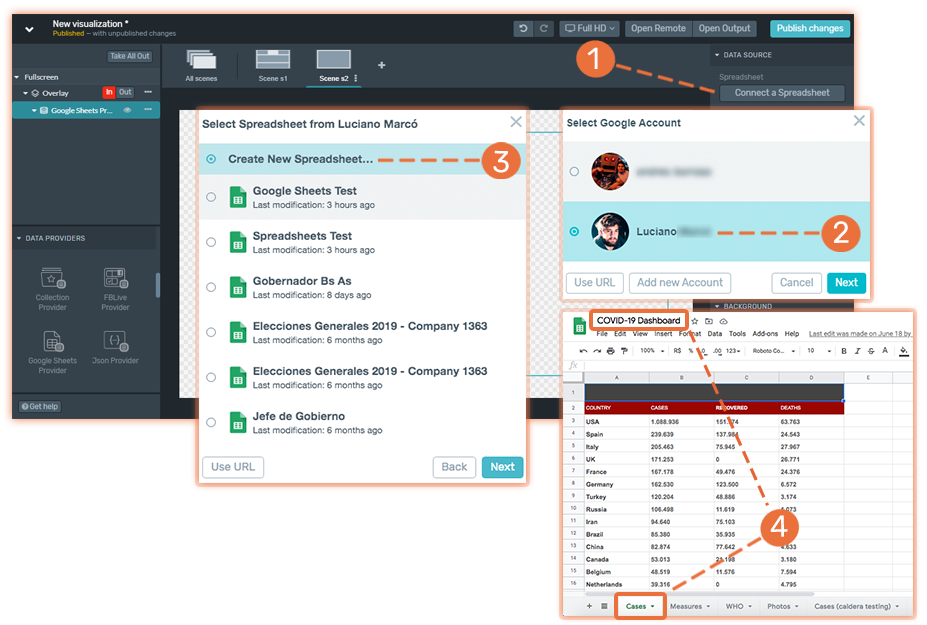
Creating a Spreadsheet:
(1) Connect a Spreadsheet.
(2) Select an account.
(3) Create a New Spreadsheet.
(4) Name the spreadsheet and sheet.
It could happen that you may not have connected a Google Account to Flowics yet, or your account is linked but Google Drive access is not enabled. Follow this steps if you don't see the required account listed:
2. After adding your account, click on Enable Google Drive Access. Keep in mind that Flowics ONLY has access to spreadsheets created within the system and will not access other files stored in your Drive.

Listed spreadsheets
Listed spreadsheets
If you have already created a Spreadsheet using this Data Provider, it will appear listed, allowing you to reuse it for a different visualization or widget.
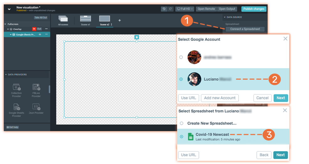
To use it:
(1) Connect a Spreadsheet.
(2) Choose the account.
(3) Find and choose the listed Spreadsheet.
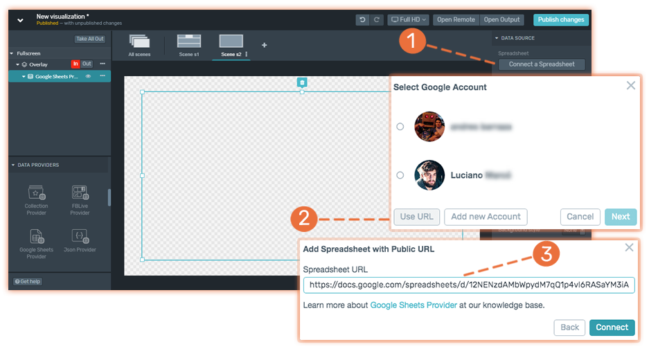
Use URL
Use URL
If you prefer not to connect your Google Account, you can connect a Spreadsheet using its URL. Just ensure the file has public access.
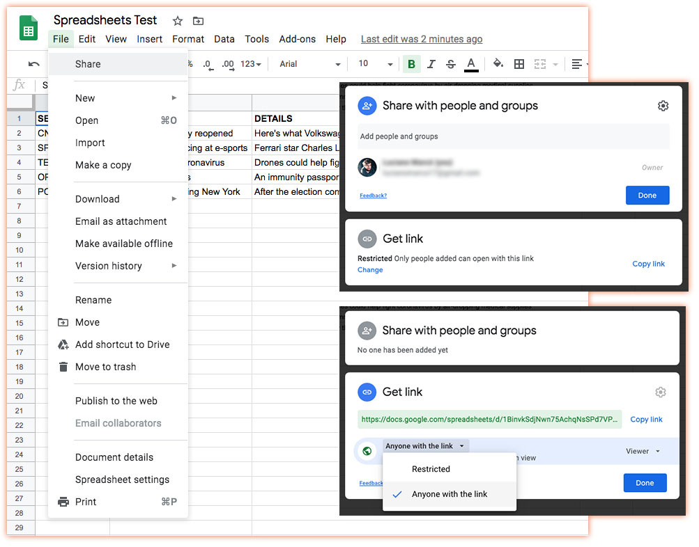
Make a Google Spreadsheet public:
Click File > Share > Get link change.
Set access to "Anyone with the link".
2. Select a Sheet

Once you have your Spreadsheet connected, you need to select the sheet you would like to work with.

(1) Choose a sheet from the list of available sheets.
(2) Click "Connect" to make the data accessible for binding with Building Blocks to create your graphics.
3. Data Binding
Bear in mind, when selecting a range of cells from the Inspector make sure all the values from each column have the same data type (numbers, date, time, image). Otherwise they will be considered as strings (as simple text). The Viz Flowics connector analyzes the data within the selected range to classify the field as either a string or a boolean:
String Classification: If the range includes any rows with string values (e.g., a header row or text in the column), the connector classifies the column as a string. As a result, conditionals for this field will appear as string comparisons.
Boolean Classification: If the range contains only formula-evaluated boolean values (TRUE/FALSE) and no strings, the connector identifies the field as a boolean. This enables boolean conditionals and toggles. To ensure boolean detection, define the dynamic list range so it excludes header or text rows and includes only rows whose formulas evaluate to TRUE/FALSE.
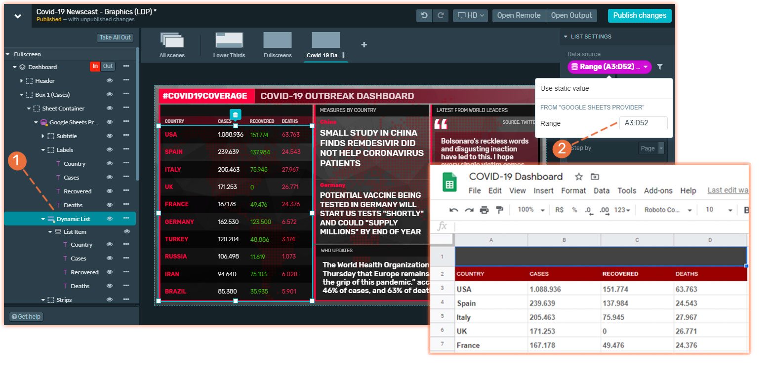
You can bind a specific cell to a node and, for the case of Dynamic Lists, you can bind a data range to use its columns as Data.
Binding Columns in Dynamic lists Use it to display a range of cells. With this selection, you can build charts with sports statistics, visual dashboards with breaking news, and more! (1) Add a Dynamic Content List as a child of the Data Provider in the tree. The list items defined in the tree will be the data placed as rows in your sheet. (2) Input the cell range that contains the data you want to display. Describe that range using this format A1:B2 (3) Add a Text Element. (4) Bind it to a specific column to display the data from each of the rows in that column. (5) Alternatively, you can choose to bind to a specific cell reference. In this case, the data will be repeated for each of the Items in your Dynamic list. Add as many Text elements as columns you want to bind.
Common Issues and Their Causes
A common issue occurs when a field intended to be boolean is misclassified as a string. This typically happens when:
The selected range includes a header row or other non-boolean text.
The column contains mixed data types, such as both text and boolean values.
Solutions for Correct Data Type Detection
To avoid misclassification:
Adjust the Data Range: Ensure the selected range excludes any rows with text or headers and includes only rows with boolean-evaluated formulas.
Verify Data Consistency: Check that all rows in the range contain consistent data types (e.g., only TRUE/FALSE values).

Data Type Recognition in Dynamic Lists
Workarounds for Misclassified Fields
If a field is classified as a string but you need boolean-like conditional visibility, you can use a workaround:
Set a conditional that explicitly checks for the boolean string value. For example, configure the conditional visibility to "is equal" = TRUE. This functions equivalently to using a TRUE/FALSE toggle on a boolean variable when the column is classified as a string.
By following these guidelines and workarounds, you can ensure that your dynamic lists in Viz Flowics function as intended, regardless of data type classification.
Binding Columns in Dynamic lists
Binding Columns in Dynamic lists
Use this method to display data from multiple cells and build charts with sports statistics, visual dashboards with breaking news, and more.
(1) Add a Dynamic Content List as a child of the Data Provider in the tree.
Each list item corresponds to a row in your spreadsheet.
(2) Input the cell range to define the data to display. Describe that range using this format A1:B2
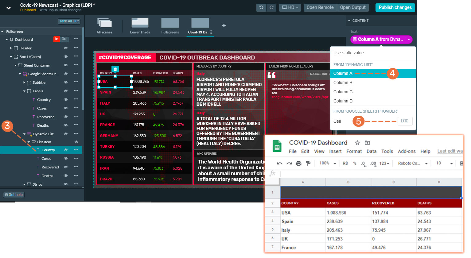
(3) Add a Text Element.
(4) Bind it to a specific column to display its data for each row.
(5) Alternatively, you can choose to bind to a specific cell reference. In this case, the data will be repeated for each item in the Dynamic List.
Add a Text elements for each columns you want to bind.
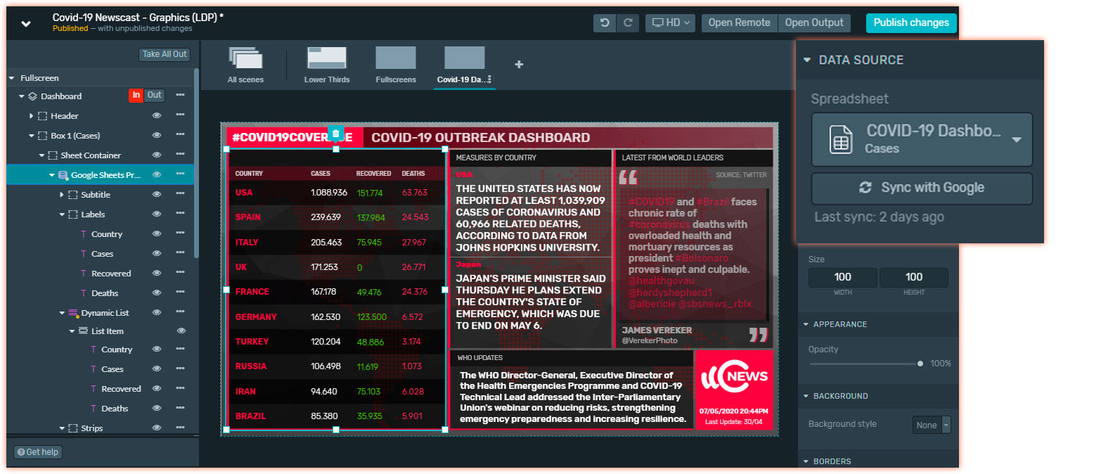
4. Sync with Google
Syncing is not automatic. If you make changes to your Google Spreadsheet, click "Sync with Google" to update the data. You can Sync either from the Graphics editor or the Remote Control.
Graphics Editor
Graphics Editor
Syncing in the Graphics Editor only updates the editor's preview, it does not affect the Live Visualization.
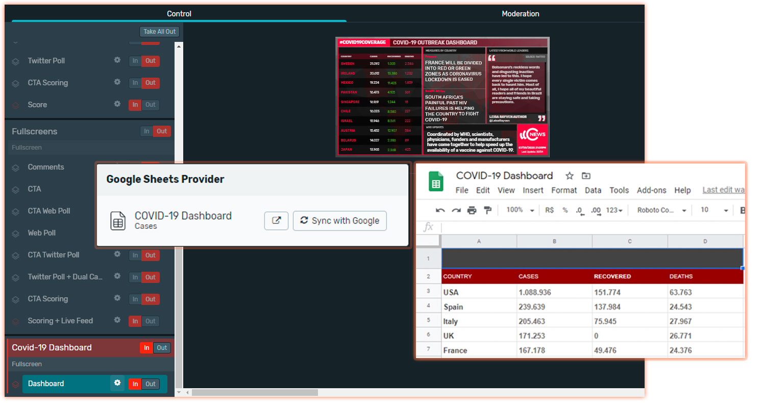
Remote Control
Remote Control
Changes made to your spreadsheet during live operation must be synchronized from the remote control so that they are reflected in the live visualization.
If you face a problem while syncing, please check our Sheets Troubleshooting article.
5. Inspirational Use Cases
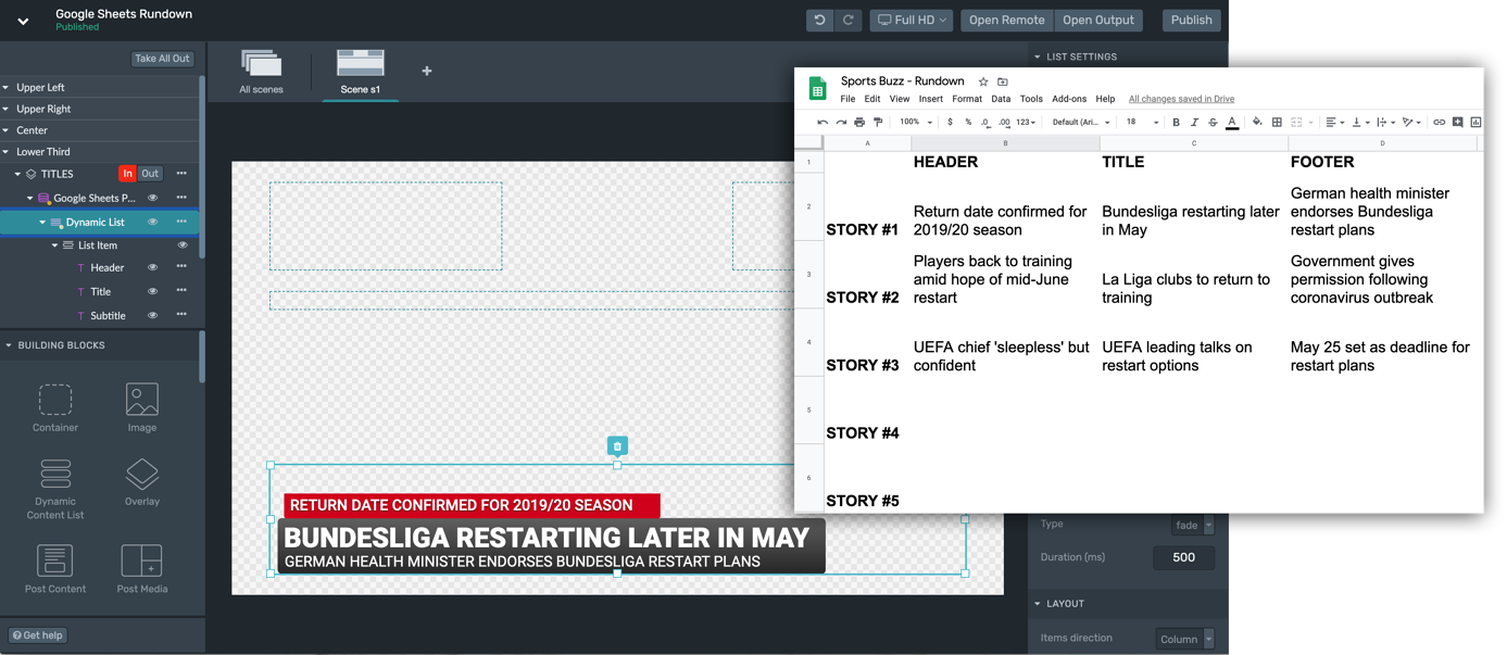
Titles and Texts as part of the Rundown
Titles and Texts as part of the Rundown
Sports Statistics & Team Lineups
Sports Statistics & Team Lineups